Plots

Defines some circadian data science plots, like actograms

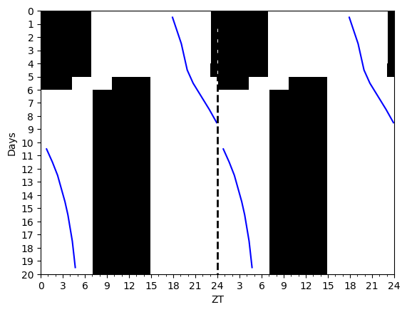
Actograms

Actograms help display periodic trends in data.

Note

I prefer my actograms to show low values as black and high values as white. The convention in circadian science (for some reason) is the reverse. This can easily be switched in plot calls if you want to do things the wrong way.

slam_shift = LightSchedule.SlamShift() 
time = np.arange(0, 20*24.0, 0.10)
light_values = slam_shift(time) 

act = Actogram(time, light_vals=light_values, smooth=False)

spm = Hannay19()
trajectory = spm(time, np.array([1.0, np.pi, 0.0]), light_values)
dlmo = spm.dlmos()

act.plot_phasemarker(dlmo, color='blue')
plt.show()

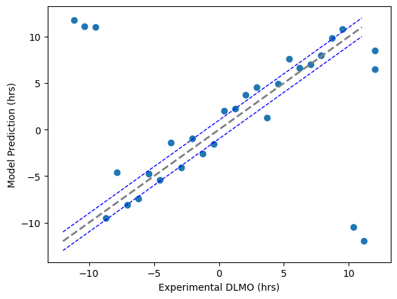
dlmo_experimental = np.linspace(-12, 12., 30) 
dlmo_predicted = dlmo_experimental + np.random.normal(0, 2, len(dlmo_experimental))

plot_mae(dlmo_experimental, dlmo_predicted)

The MAE is: 4.893222072754772
Within one hour 7/30
[-3.47328784e+00  2.29203680e+01  2.14370972e+01  2.05151476e+01
 -8.28809784e-01  3.29152432e+00 -1.03521731e+00 -1.21786907e+00
  6.01046181e-01 -8.64421152e-01  2.32069554e+00 -1.20140297e+00
  1.11533503e+00 -1.35758354e+00 -1.13861312e+00  1.62675565e+00
  1.03264169e+00  1.65883693e+00  1.66964836e+00 -2.41250659e+00
  3.98410068e-01  2.24680534e+00  4.61070620e-01 -1.11127185e-02
  8.78906427e-02  1.18376113e+00  1.25223210e+00 -2.07873084e+01
 -2.31041479e+01 -5.54511532e+00]

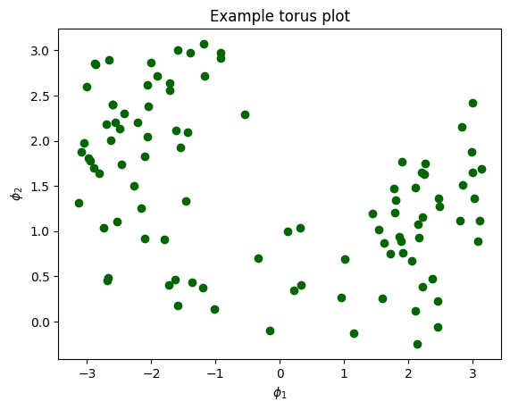
Here is an example of the torus plot, which allows one to visualize the relationsjip between two phases.

phi1 = 12.0 + 5.0*np.random.randn(100) 
phi2 = phi1 + 5.0*np.random.randn(100)

plot_torus(phi1, phi2, scaled_by=24.0, color='darkgreen')
plt.title("Example torus plot")
plt.xlabel("$\phi_1$") 
plt.ylabel("$\phi_2$");

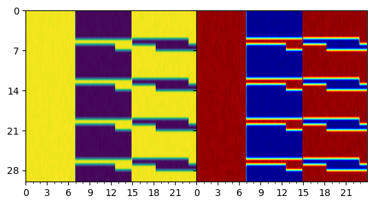
Example of an actogram

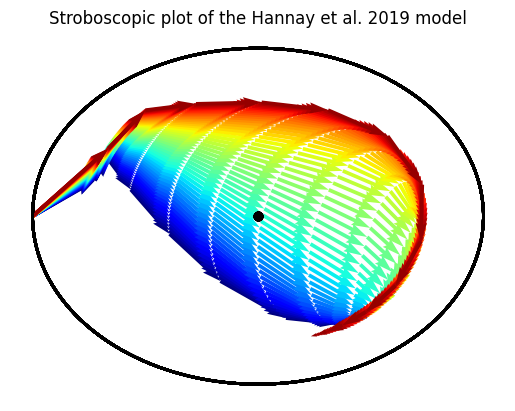
This is how you can visualize entrainment using a Stroboscopic plot of a trajectory

slam_shift = LightSchedule.SlamShift(shift=12.0, lux=500.0, before_days=2) 
time = np.arange(0.0, 15*24.0, 0.10)
light_values = slam_shift(time)
# Run this for a range of period parameters 
batch_dim = 50
hmodel = Hannay19({'tau': np.linspace(23.5, 24.5, batch_dim)}) 

initial_state = np.array([1.0, np.pi, 0.0]) + np.zeros((batch_dim, 3))
initial_state = initial_state.T
trajectory = hmodel(time, initial_state, light_values)

ax = plt.gca()
cmap = plt.get_cmap('jet')
for idx in range(trajectory.batch_size):
    Stroboscopic(ax, 
                 time, 
                 trajectory.states[:, 0, idx], 
                 trajectory.states[:, 1, idx], 
                 period=24.0, 
                 lw=0.50,
                 color=cmap(idx/batch_dim));
plt.title("Stroboscopic plot of the Hannay et al. 2019 model");

slam_shift = LightSchedule.ShiftWork() 
time = np.arange(0, 30*24.0, 0.10)
light_values = slam_shift(time) + np.random.randn(len(time)) * 1.0

fig, ax = plt.subplots(1, 2, sharey='row')
act = plot_actogram(ax[0], zeitgeber=light_values, cmap='viridis')
act = plot_actogram(ax[1], zeitgeber=light_values)

fig.subplots_adjust(wspace=0, hspace=0)